Give us a call

Ferrum Technology Services Blog

Ferrum Technology Services has been serving the Elgin area since 2007, providing IT Support such as technical helpdesk support, computer support, and consulting to small and medium-sized businesses.

How to Get Your Spreadsheets to Accurately Add Time
How to Get Your Spreadsheets to Accurately Add Time

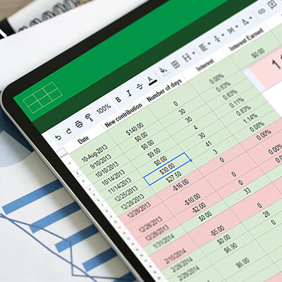
Handling time calculations in a spreadsheet can often feel frustrating—especially when you’re just trying to add them up. Luckily, both Microsoft Excel and Google Sheets have built-in functions specifically designed for this purpose, making the process more manageable.

Here’s a quick guide to help you get started, no matter which spreadsheet program you use.

How to Use the Dynamic Time Function for Time Calculations

While relying on a specialized formula to add times may seem complex at first, it actually gives you more precise control over your calculations, ensuring your time sums are both accurate and practical.

To use the Dynamic Time Function, you need to start with an initial time value. Let’s say we use 12:00:00 AM, ensuring the data is formatted as "Time." In Excel, this can be adjusted from the Home menu in the dropdown box above Number, while Google Sheets has the adjustment in the Format menu, where you find the Number option and Time can be selected.

Now, let’s break down the formula. For simplicity, we’ll assume we’re working in row one, starting with cell A1:

=A1+TIME(0,0,0)

In this formula, A1 contains your starting time, while the TIME function breaks the adjustments into hours, minutes, and seconds. Since we haven’t made any changes yet, both A1 and the result cell would show 12:00:00 AM.

Next, you’ll want to replace the zeroes in the formula with actual time values. These values can be drawn from other cells to sum up the total time. Your formula might then look like this:

=A1+TIME(B1,C1,D1)

Here, B1, C1, and D1 represent the number of hours, minutes, and seconds you want to add to the time in A1. For example:

If A1 starts at 12:00:00 AM, and B1, C1, and D1 are populated with 2, 4, and 6, your result will be 2:04:06 AM.

If B1 is 9 and D1 is 38, your final time will be 9:04:38 AM.

It might feel tricky at first, but once you get the hang of it, the Dynamic Time Function can be a powerful tool—whether you’re calculating deadlines or estimating the completion of tasks or processes.

Return to our blogs soon for more great tips and tricks using some of today’s most popular productivity tools like Microsoft Excel.

Tip of the Week: How to Share Large Files
Three Ways SMBs Combat Mobile Malware
 

Comments

No comments made yet. Be the first to submit a comment
Guest
Already Registered? Login Here
Guest
Wednesday, 22 January 2025

Captcha Image

Blog Archive

2025
February
March
April
May
June
July
August
September
October
November
December
2012
January
February
March
April
May
June
July
August
September
October
November
December
2011
January
February
March
April
May
June
July
August
September
October
November
December
2010
January
February
March
April
May
June
July
August
September
October
November
December
2009
January
February
March
April
May
June
July
August
September
October
November
December
2008
January
February
March
April
May
June
July
August
September
October
November
December
2007
January
February
March
April
May
June
July
August
September
October
November
December

Mobile? Grab this Article

QR Code

Contact us

Learn more about what Ferrum Technology Services can do for your business.